

Jupyter notebooks are an essential part of every data analyst’s toolkit. They allow you to code and iterate through different models quickly, publish your process and results for easy reproducibility, and help you create compelling visualizations and narratives to accompany your analytical findings.
As Jupyter notebooks would typically be your first entry point in learning how to do data analytics and data science, we first provide some context for understanding why notebooks are important for exploratory analysis, before diving into a practical example of how we can install, create, and work with them.
Are you excited to learn more about how Jupyter notebooks can accelerate your analytics process? Read on to find out!
In programming, notebooks refer to something very different from your everyday paper notebook. Computational notebooks have become an increasingly popular way in which you can write and run computer programs, create calculations, and produce visualizations.
Jupyter notebooks are a specific type of computational notebook. It was previously known as IPython but was spun off as a separate entity. Jupyter notebooks are one of the most popular notebooks in use today. A study in 2018 found that there were more than 2.5 million publicly accessible Jupyter notebooks.
They are free, open-source, and you can use them with three popular languages that make up the name of the tool: Julia (Ju), Python (Py) and R. SageMaker Notebooks (Amazon), Colaboratory (Google), and Azure Notebook (Microsoft), are examples of how large companies have also adopted its use in their offerings.
Because Jupyter notebooks support code, text, and images, they provide a flexible and ideal way to manage the iterative exploration process common to data analytics and machine learning. They also allow you to document your process and present your findings within the same format, reducing the need to transfer your key findings into a slide deck or report. Furthermore, you can easily rerun code in a notebook published by someone else to verify their calculations and methodology for yourself, and modify it by editing the code directly to suit a different dataset’s needs.
These attributes are in fact some of the reasons why notebooks are often the first tool that data analysts will reach for when presented with a new project or dataset to analyze. Several business intelligence companies like Hex , Mode , and Tableau have begun to integrate notebooks into the data analytics workflow.
To get a sense of what’s possible with a Jupyter notebook, it’s worth browsing notebooks that have been published online. For example, check out the Python Data Science Handbook . You can read the code from the handbook in this repository of Jupyter notebooks that includes explanations with each code cell, and you can even run the code yourself locally or in the cloud, which we’ll show you how to do below. Amazon Web Services also shares examples of Jupyter notebooks on how to run machine learning models entirely through a notebook.
More advanced users can run Jupyter notebooks locally. We’ll follow the official guide here from Project Jupyter. You will first need to install Python as it’s a necessary prerequisite for Jupyter notebooks. You can either do this through installing Anaconda, which will handle the installation of Python and Jupyter notebook for you, or through using pip, Python’s package manager, in your local terminal.
While Project Jupyter recommends using Anaconda, there are pros and cons with either approach. Anaconda has a more user-friendly, GUI-like interface, and will walk you through the entire process, but it comes with more than 700 packages, which takes up a lot of space in your computer. With pip, running commands via your local terminal can seem scary if you’ve never done it before, but the commands are quite simple and you can copy and paste them from the guides. Pip lets you install only the packages that you will be using, and the process lets you get up and running much faster too.
Installing via Anaconda
Installing via pip
The easiest way to get started with Jupyter notebooks is to use Google Colab instead of installing it locally.
It allows users to get up and running within seconds, which can be helpful for beginners as it can be more challenging to learn how to install Project Jupyter and connect the correct kernels to run a Jupyter notebook locally. Google Colab does not require you to set up your environment beforehand either. This is a great way in which you can become familiar with how notebooks work before moving on to more advanced use cases.
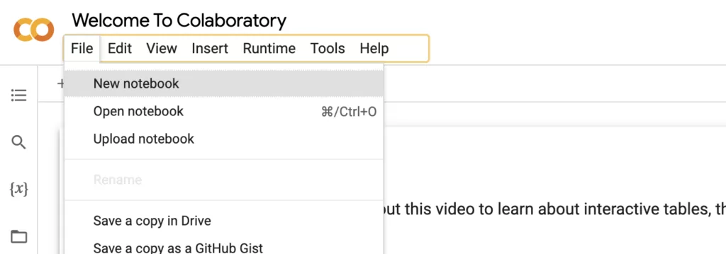
Head over to Google Colab to get started. Under File, click on New notebook to launch your very first Jupter notebook in new tab:
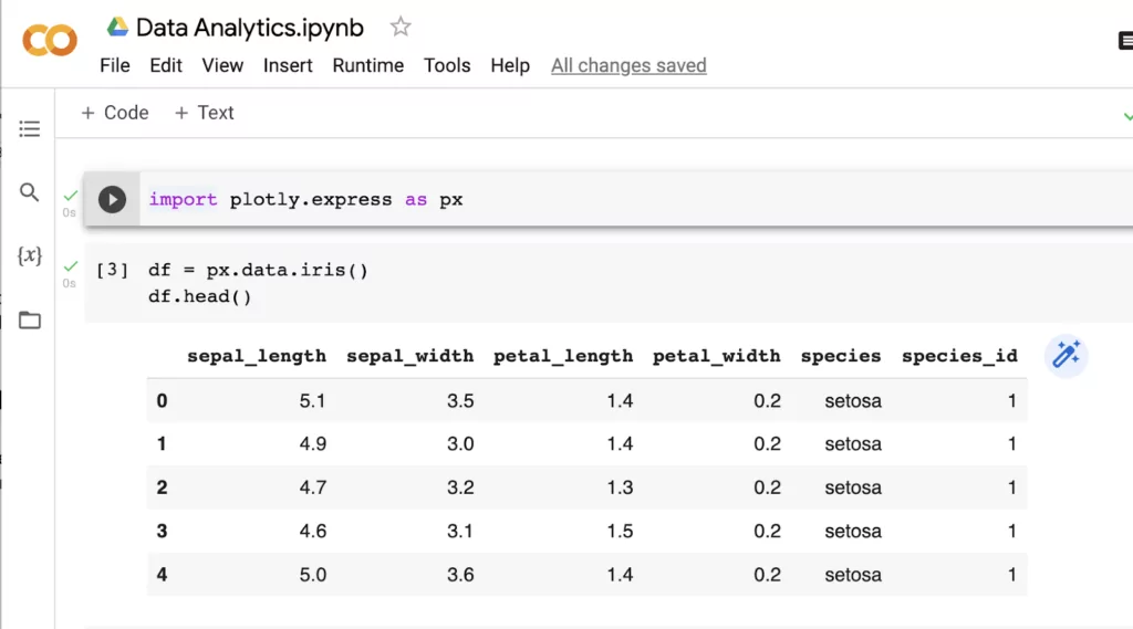
Now, give your notebook a name. Jupyter notebooks end with a .ipynb extension as they are a JSON file. You can see that you can create ‘Code’ or ‘Text’ blocks, the play button allows you to run code blocks to execute your code:

These code cells let you execute code in the kernel. Cells are where you write your code (or text, if you choose a Markdown cell instead). A kernel is what enables you to run the code you have in your notebook. They’re a bit more complicated to understand, the main thing you need to know when you’re just starting is that you can stop a long-running computation just by hitting “Interrupt execution” under Runtime.
And that’s it! In just two clicks, you’re ready to start analyzing data. To do that, we’ll use a basic visualization example from Plotly as a way to walk through how you can use your notebook for easy and efficient analysis.
Let’s take a look at this example on how to create an informative visualization of the Iris dataset, an essential step before we can perform Principal Component Analysis (PCA).
In the first code block, we’ll import any dependencies we might need. In this example, we’re only working with Plotly Express, but more advanced projects will involve more installations. Then, we’ll read in the Iris dataset into a dataframe and take a look at the first few rows to get a sense of what the data looks like:
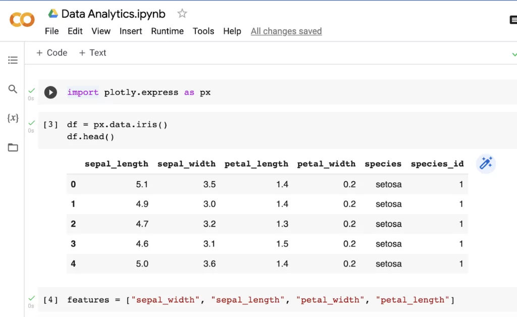
There are more attributes here than we will need, so we’ll filter the dataset to only include these columns:
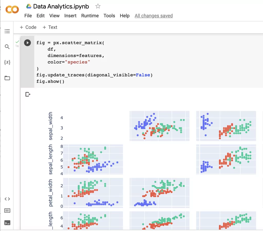
Then, we’ll create a simple scatter plot with a matrix of each attribute. Once you click run on the code block, the visualization appears.
Now that we have some basic analysis ready to share with others, let’s tidy it up and add some Markdown formatting to help our readers understand what we are trying to accomplish with our notebook:
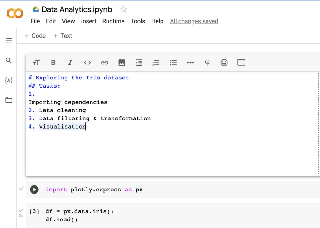
Markdown is a language that helps us format text with different heading levels, bullet points, lists, links, inline coding, and adding images. Once you run the cell, it looks like this:
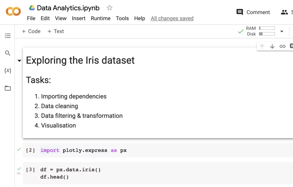
Your first notebook is done! How do you go about sharing it? We recommend using NBViewer to publish and render your notebook online. After you upload your notebook on GitHub and paste the link in NBViewer, you’ll be able to get a URL to share your work with anyone in the world.
There are also some neat, time-saving shortcuts you can learn to make the coding process run more smoothly. Use control-enter to run the cell, option-return to run the cell & add a new code block below, and esc-d-d to delete the current code block.
We hope that this article has helped you understand Jupyter notebooks better. As notebooks have become a key part of the data analytics workflow for data teams at top companies worldwide, it is beneficial to gain a deeper understanding of it by trying it out yourself.
Let’s quickly review how you can best make use of Jupyter notebooks in your next project:
Has this Jupyter Notebook tutorial piqued your interest in learning more about analytics roles and the field of data analytics in general? Why not try out this free, self-paced data analytics course ? You may also be interested in the following articles:
This article is part of:
Writer for The CareerFoundry Blog
Elliot is a technical writer specializing in data engineering and data science. He recently completed his MSc. in Economic History at the London School of Economics, and has worked at Plotly and Towards Data Science. When not coding or writing about code, he enjoys coaching LEGO robotics.


CareerFoundry is an online school for people looking to switch to a rewarding career in tech. Select a program, get paired with an expert mentor and tutor, and become a job-ready designer, developer, or analyst from scratch, or your money back.